|| Communicating Science || An enterprise of the Invariance Publishing House, a journal with a difference of the || MDash Foundation ||
Sunday, November 4, 2012
Tuesday, September 11, 2012
Sunday, February 5, 2012
Heisenberg's Uncertainty Principle from a new angle
------------------------------------------------------------------- Blogs Here
---------------------------------------------------------------------------------
Heisenberg's Uncertainty Principle from a new angle
---------------------------------------------------------------------------------
This is a draft of an unfinished blog
Heisenberg's Uncertainty Principle from wave-particle duality. The wave-particle duality states that any mechanical object can exhibit both wave and particle behavior and the complementarity priniciple states that they can not both be observed simultaneously. That is the wave and teh particle nature are only exclusive ly observed given a specific time or time window, the window being consistent with Heisenberg's uncertainty prinicples of which there are more than 3 forms. But only 3 forms of these exhibit a simple relation from which other-varable relationships can be derived much in the same way kinetic energy is derived from mass and speed of a particle. The intention of writing this blog for me is to show how a basic reasoning can be applied qualitatively to obtain a semi-quantitative or intuitive relation between variables to extend an inequality relation between these variables. I will show here only for energy and time uncertainty relationship. From the wave particle duality it is clear that any entity/object/process has a particle or wave character both in the same system but not in the parametric sense of same time. Once time is chosen/defined as a specific kinematic parameter wrt that time the wave and particle nature are not simultaneously observed. So let us consider a particle, say a neutrino or an electron. This particle has a well specified physical location in space. This is the mean position therefore of the particle. This mean has a zero distribution for a classical particle but for a quantum mechanical particle or system the distribution is not zero. Now the particle also being a wave it has a characteristic of wavelength. This wavelength therefore gives the extent of deviation of the particle's position from its mean location. The wavelength is lambda.
Blogs here is a blogging page on "Communicating Science" which is the home page of the current website scicomn.blogspot.com,
---------------------------------------------------------------------------------
If you want to post a blog of interest to science please send an email to Manmohan Dash: g6pontiac@gmail.com.
---------------------------------------------------------------------------------
---------------------------------------------------------------------------------
If you want to post a blog of interest to science please send an email to Manmohan Dash: g6pontiac@gmail.com.
---------------------------------------------------------------------------------
---------------------------------------------------------------------------------
Heisenberg's Uncertainty Principle from a new angle
---------------------------------------------------------------------------------
This is a draft of an unfinished blog
Heisenberg's Uncertainty Principle from wave-particle duality. The wave-particle duality states that any mechanical object can exhibit both wave and particle behavior and the complementarity priniciple states that they can not both be observed simultaneously. That is the wave and teh particle nature are only exclusive ly observed given a specific time or time window, the window being consistent with Heisenberg's uncertainty prinicples of which there are more than 3 forms. But only 3 forms of these exhibit a simple relation from which other-varable relationships can be derived much in the same way kinetic energy is derived from mass and speed of a particle. The intention of writing this blog for me is to show how a basic reasoning can be applied qualitatively to obtain a semi-quantitative or intuitive relation between variables to extend an inequality relation between these variables. I will show here only for energy and time uncertainty relationship. From the wave particle duality it is clear that any entity/object/process has a particle or wave character both in the same system but not in the parametric sense of same time. Once time is chosen/defined as a specific kinematic parameter wrt that time the wave and particle nature are not simultaneously observed. So let us consider a particle, say a neutrino or an electron. This particle has a well specified physical location in space. This is the mean position therefore of the particle. This mean has a zero distribution for a classical particle but for a quantum mechanical particle or system the distribution is not zero. Now the particle also being a wave it has a characteristic of wavelength. This wavelength therefore gives the extent of deviation of the particle's position from its mean location. The wavelength is lambda.
Saturday, January 28, 2012
Radioactivity of cigarettes and banana
Citation: "Radioactivity of cigarettes and banana", Manmohan Dash, Communicating Science, April 11, 2011, publisher: Invariance Publishing House, MDash Foundation
Link to permaweblink in citation or copy/archive material as it is with Creative Commons and other copyrights in this web-site in mind: permaweblink
Link to permaweblink in citation or copy/archive material as it is with Creative Commons and other copyrights in this web-site in mind: permaweblink
Radioactivity of cigarettes and banana
Manmohan Dash
First publicized/Available Online (Article-1, Article-2): Mar 28, 2011, April 1, 2011
1 Activity of Cigarettes
Units: 37 GBq = 37×109 Bq = 1 Curie, Radioactivity of Pb (210) and Po (210): Lead 210, 22.3 years, 207.2 g ⁄ mol … Q = 0.064 MeV (β), Polonium 210, 137.376 days, 210 g ⁄ mol … Q = 5.407 MeV (α). Let’s assume the amount of Lead and Polonium to be 0.5 micro-gram each in 1 cigarette. So

mol of Pb and

mol of Po. 1 mol = 6.022 × 10²³ “elements”. This implies

nuclei of Pb is 1.45 × 10¹⁵ ⁄ cigarette. This in turn implies 6.022 × 1017 × (0.5)/(210) nuclei of Po is 1.43 × 10¹⁵ ⁄ cigarette. Activity: Pb: (1015 × 1.45 × 0.693)/( 22.3 × 365 × 24 × 3600) = 1.43 × 10⁶ decays ⁄ second = 1.43 MBq = (0.00143)/(37). Units: Curies = 38.65 microCurie, Po: 1015 × 1.43 × 0.693 × 137.376 × 24 × 3600 = 8.35 × 10⁷ decays ⁄ second = 83.5 MBq = (0.0835)/(37) Curies = 2.26 milliCuries. So the β energy of the Pb (210) makes it 1.43 MBq × 0.064 MeV = 91.52 GeV = 91.52 GeV ⁄ cigarette = 91.52 × 109 × 1.6×10 − 19J = 14.64 nanoJ ⁄ cigarette.
Or 14.64 nanoGray ⁄ cigarette, considering 1 kg of absorbing material = 1.76 nSv ⁄ cigarette. Considering 20 cigarettes a day, that is, a pack of cigarettes, and regular smoking through a year this would be 20 × 365 × 1.76 nSv = 12.83 microSv ⁄ year. Lung has a weighing factor of 0.12 and Beta (β) emission has a weighing factor of 1. So Po(210) with α emission would be 83.5 MBq × 5.407 MeV which is actually 4.51 × 10⁵ GeV = 4.51 × 1014 × 1.6 × 10 − 19 J = 72.2 microJ ⁄ cigarette. Or 72.2 microGray ⁄ cigarette = 8.664 microSv ⁄ cigarette. So with a pack of 20 cigarettes and 365 days of smoking one would collect a dose of 20 × 365 × 8.664 microSv = 63.247 milliSv ⁄ year.
This is considering 1 kg of absorbing material, lung’s radiation damage factor and a simple α emission effect not considering α emission nuclear recoil. Also I have not multiplied the factor 20 for α − particles which is prescribed, since I already calculated the energy I am not sure its necessary or not. In any case its dangerous enough. Po is more dangerous than Pb for lung cancer. If the cigarette would indeed contain 0.5 micro − gram of Pb and Po, which is not known a priori, the values from experiment performed, 2 examples shown below shows different value, which just means the cigarettes contain correspondingly different radioactive contents, which is nonetheless harmful enough to kill smokers by lung cancer.
mol of Pb and
mol of Po. 1 mol = 6.022 × 10²³ “elements”. This implies
nuclei of Pb is 1.45 × 10¹⁵ ⁄ cigarette. This in turn implies 6.022 × 1017 × (0.5)/(210) nuclei of Po is 1.43 × 10¹⁵ ⁄ cigarette. Activity: Pb: (1015 × 1.45 × 0.693)/( 22.3 × 365 × 24 × 3600) = 1.43 × 10⁶ decays ⁄ second = 1.43 MBq = (0.00143)/(37). Units: Curies = 38.65 microCurie, Po: 1015 × 1.43 × 0.693 × 137.376 × 24 × 3600 = 8.35 × 10⁷ decays ⁄ second = 83.5 MBq = (0.0835)/(37) Curies = 2.26 milliCuries. So the β energy of the Pb (210) makes it 1.43 MBq × 0.064 MeV = 91.52 GeV = 91.52 GeV ⁄ cigarette = 91.52 × 109 × 1.6×10 − 19J = 14.64 nanoJ ⁄ cigarette.
Or 14.64 nanoGray ⁄ cigarette, considering 1 kg of absorbing material = 1.76 nSv ⁄ cigarette. Considering 20 cigarettes a day, that is, a pack of cigarettes, and regular smoking through a year this would be 20 × 365 × 1.76 nSv = 12.83 microSv ⁄ year. Lung has a weighing factor of 0.12 and Beta (β) emission has a weighing factor of 1. So Po(210) with α emission would be 83.5 MBq × 5.407 MeV which is actually 4.51 × 10⁵ GeV = 4.51 × 1014 × 1.6 × 10 − 19 J = 72.2 microJ ⁄ cigarette. Or 72.2 microGray ⁄ cigarette = 8.664 microSv ⁄ cigarette. So with a pack of 20 cigarettes and 365 days of smoking one would collect a dose of 20 × 365 × 8.664 microSv = 63.247 milliSv ⁄ year.
This is considering 1 kg of absorbing material, lung’s radiation damage factor and a simple α emission effect not considering α emission nuclear recoil. Also I have not multiplied the factor 20 for α − particles which is prescribed, since I already calculated the energy I am not sure its necessary or not. In any case its dangerous enough. Po is more dangerous than Pb for lung cancer. If the cigarette would indeed contain 0.5 micro − gram of Pb and Po, which is not known a priori, the values from experiment performed, 2 examples shown below shows different value, which just means the cigarettes contain correspondingly different radioactive contents, which is nonetheless harmful enough to kill smokers by lung cancer.
Since from the experiments of “Khaterl”(REF-I↓) and “Papastefanou”(REF-II↓) below, we have an annual dose of 100 microSv on an average for radio-active Pb as well as Po, it just means that we have more than 0.5 micro − gram of Pb but less than 0.5 micro − gram of Po in a single cigarette. Po is highly radio-active (Po − 210 has a much smaller half-life) and emits α − rays, therefore much more dangerous than Pb − 210.
2 Activity of Bananas
Bananas Are Radioactive
Anne Marie Helmenstine [Ph.D., About.com Guide]
Source: Chemistry, About.Com
Excerpt/Abstract: from above article:
“Bananas are radioactive for a similar reason. The fruit contains high levels of potassium. Radioactive K-40 has an isotopic abundance of 0.01% and a half-life of 1.25 billion years. The average banana contains around 450 mg of potassium and will experience about 14 decays each second. It’s no big deal. You already have potassium in your body, 0.01% as K-40. You are fine. Your body can handle low levels of radioactivity.”
- JOE: so the half life is 1.25 billion years and decays 14 times a second? are you sure you know what your talking about?
- AMASA @joe: There are many, many, many, many, many molecules of potassium in 450 mg of potassium.
- CHRIS @joe, the math looks a bit off, but not in the way you’re thinking, so let me break it down. half life of K − 40 = 1.248 × 10⁹ years years, natural abundance of K − 40 = 0.012, molar mass of K − 40 = 39.96399848 g ⁄ mol, 450 mg × 0.012, 5.4 mg = 0.0054 g, (0.0054 g)/(39.96399848 g ⁄ mol) = 1.3512 × 10 − 4 mol, 1.3512 × 10 − 4mol × 6.022 × 1023particles ⁄ mol = 8.137 × 10¹⁹atoms, K − 40, 4.0685 × 10¹⁹ decay in the first 1.248 × 10⁹ years, average of 3.26 × 10¹⁰ per year, average of 1033 ⁄ second
- MARK ANDERSON @Chris Close, but its .012 which is really 0.00012 which works out to about 0.054 mg.
- ELIOT Good work Chris and Mark. However your estimate for number of decays per second will be off because you didn’t figure them using logs. Radioactivity is an exponential decay function. So the number of decays per time unit starts higher and then slowly gets lower over time. So one second now will have almost twice as many decays as one second 1.248 × 10⁹ years from now. Of course we are interested in the rate of decays for seconds now not 1 billion years in the future. This is what pushed the number to 14 per second.
- MANMOHAN DASH [ independent work of Manmohan Dash] Hi Chris, Mark: you laid the ground work. Thanks. I will complete the calculation and show you this is exactly rounded to 14 decays per second. If you change your fraction of radioactive K − 40 to 0.01 as in the article rather than 0.012 etc I think it will give the exact answer. Here is the answer: I take the calculation you two have done correctly, i.e. the 450 milligram banana contains 8.137 × 10¹⁷ nuclei of K − 40 (not 1019 as corrected by Mark) Now the decay constant or transition probability as one may call it which gives the probability at any time of a single nucleus to decay at any time is ω = (0.693)/(Thalf − life). This is obtained by using Heisenberg Uncertainty principle for the nuclear decay. Here decay width which is given as a width of energy and mean life time which is given as a width or uncertainty in time, must multiply to h-cross (time - energy uncertainty). Now Mean life is related to half-life by the factor 0.693 (69.3% of nucleus would decay in the mean life where as 50% would decay in a half-life) So the decay probability = ω gives the probability or likelihood that any single nucleus will decay or not. So we know this probability because we know the half life to be 1.25 billion years that is 1.25 × 365 × 24 × 3600 × 109seconds = 1.25 × 3.15 × 1016seconds. Since the banana has450 milli − grams of Potassium it has as many radioactive K − 40 as we just counted, 8.137 × 10¹⁷ nuclei, at the time of eating. So the probability of decay is ω and you know how many nuclei you got. Multiply them to get the exact number of radioactivity of your banana. Needless to say this product is 14.3.(8.137 × 0.693)/(1.25 × 3.15 × 1017 − 16) = 1.43 × 10 = 14.3.
References:
I haven't read these papers, only the abstract available to me as these are paid for publications
Ref-I [License info]
Polonium-210 budget in cigarettes
Ashraf E.M Khater
National Center for Nuclear Safety and Radiation Control, Atomic Energy Authority, P.O. Box 7551, Nasr City, Cairo 11762, Egypt
Ref-II [Open Access]
Papastefanou, C. Radioactivity of Tobacco Leaves and Radiation Dose Induced from Smoking. Int. J. Environ. Res. Public Health 2009, 6, 558-567.
Corresponding author: papastefanou@physics.auth.gr
Tuesday, January 17, 2012
Article: Doppler Shift and Time Dilation, binomial analysis
FYI-1: This version is being reviewed for correct html rendering.
FYI-2: our paper version on Philica.com, cited below, has some errors in Note-3. The Note-3 in this html version, the UTexas Math-Phys Archive version and the HAL INRIA version are correct. We have communicated with Philica to have Note-3 replaced with the correct version.
FYI-3: One obvious typographical error in earlier versions has been fixed.

((should actually be))
 .
.
The above typo is not corrected in any archive copies.
If you want to cite our version
Citation: "Time dilation have opposite signs in hemispheres of recession and approach.", Manmohan Dash and Mikael Franzen, Communicating Science, January 17, 2011, publisher: Invariance Publishing House, MDash Foundation
Our citations might slightly change depending on exact source where we placed our ideas first. eg we may want to cite our online journals "Various Musings" if we formalize it and make it permanent.
Link to permaweblink in citation or copy/archive material as it is with Creative Commons and other copyrights in this web-site in mind: permaweblink
Alternative versions
i. Dash, M. & Franzén, M. (2012). Time dilation have opposite signs in hemispheres of recession and approach. PHILICA.COM Article number 312.
ii. University of Texas, Mathematical Physics, Mathematical Physics Preprint Archive mp_arc
iii. Open Access on HAL INRIA (ps, pdf) HAL-Inria; Link to the pdf PDF version of the paper
Time dilation have opposite signs in hemispheres of recession and approach.
Manmohan Dash
mdash@vt.edu
manmohan.dash@willgood.org
i. Informal association with Willgood institute, registered in Sweden, author’s mail: Mahisapat, Dhenkanal, Odisha, India, 759001
ii. previously affiliated with VT, USA and KEK, Japan.
Mikael Franzén
mikael.franzen@willgood.org
mikael.franzen@i3tex.com
i. Willgood Institute, Luckvägen 5, 517 37 Bollebygd, Sweden
ii. i3tex AB, Klippan 1A , 414 51 Gothenburg, Sweden
Abstract
In this paper we give a detailed analysis of the factual observation that time dilation or Doppler shift of frequency are oppositely signed relative to our line of sight in different regions of motion. We show that this depends on how these regions are connected to the actual path of motion and to the location of the observer/detector. For a static globe or circle/sphere of reference, we define two hemispheres; shifts will be red-shifted in the hemisphere of recession and blue-shifted, or violet shifted, in the hemisphere of approach, a fact which is not often mentioned. Indeed, it is a complete sphere where the motion can take place with respect to the line-of-sight, which we have studied in this paper, not just the direction of motion along a certain specific path. The transverse and longitudinal effects are special cases of this general effect. The transverse effect is always red-shifted consistent with the known effect of Relativity and it lies at the intersection of the hemispheres of approach and recession. By saying moving clocks run slower we conveniently forget this important effect. They also run faster, in the hemisphere of approach. We demonstrate this important result from the basic principles of the Special Theory of Relativity.
Keywords: Time Dilation, Special Relativity, Doppler Shift, Binomial Expansion, Celestial trajectories and Time dilation
1 Introduction
We perform a detailed analysis of how relative to the line-of-sight a general motion of a source and equivalently an observer will affect observation of time dilation and Doppler shift. We use only two main references, so we mention this fact here; [Ref-1] and [Ref-2]. It is a straightforward but non-trivial analysis. It applies to any situation where one would like to have a binomial expansion of the Lorentz factors γ and β to any desired degree of accuracy by retaining terms up-to one’s requirements. This will be useful in many studies.
Let us now define the context in which we have used terminology like “sphere of relative motion”, “hemispheres of recession” and “spheres of reference”; see Figure 1↓ and Figure 2↓. Our definition is a natural extension of the concept of reference frames. This is helpful towards identification of the relations of different parts to each other in the problem. Simply put, one defines two spheres/circles, the first one is a sphere of reference whose center is where a detector or origin of reference is located. The detector can also be placed e.g. at the surface of another object whose center is at the center of this reference. Any concentric sphere that encloses or excludes a segment of the trajectory of another object is also a sphere of reference. Now a second sphere of reference can be defined. This second sphere will encompass a segment of the trajectory path so the path lies in either the lower or upper hemisphere with respect to the line of sight. Let us call it a sphere of relative motion as it defines whether an object is receding away from, or approaching the center of reference. The upper hemisphere of this second sphere, where an object is gradually moving away from the reference point, defined at the center of the first sphere, can be called a hemisphere of recession. On the other hand, if the object is in the lower hemisphere of the second sphere, we can call it a hemisphere of approach, as the object will gradually approach the center of reference. One must note that these spheres are not very arbitrary in nature, but rather, dependent on the specific nature of the trajectories, e.g. a satellite orbiting a planet in a circle will naturally always traverse the intersection of the two hemispheres, so it is a transverse motion to the line of sight. In hyperbolic motion, such as that of a flyby satellite moving away from a planet towards some other destination, part of the motion lies in the upper hemisphere or the hemisphere of recession. When dealing with earthbound motion, such as before perigee, the point of closest approach to earth, the opposite is true. The segment of the trajectory is naturally proportional to the radial speed vector. The radial − speed − vecor is very important for any study of celestial applications. Similarly a meteor falling towards Earth always lies in the hemisphere of approach. One sees that one can cautiously adjust the sphere of reference and the sphere of relative motion so that there is no ambiguity in the situation. Only then can one consistently apply the laws of Relativity, such as those that govern time dilation and Doppler shift of frequencies.
We also note as a reminder of convenience that the transverse effects are always 2nd order in speed of recession and the longitudinal effects are 1st and 3rd order in terms of the Lorentz factor, β. Higher order terms appear in the same pattern. Transverse effects contain β2 and β4 and longitudinal effects contain alternative odd terms given by factors from binomial expansion as presented in our analysis.
The general case is accommodated by cosines of a suitable angle, which appear only in the orders of odd power terms. The analysis is valid for 0 ≤ abs(β) ≤ 1, where abs stands for the modulus of a number or the regular absolute value function. The relation between fractional frequency shift fν and fractional time dilation or contraction ft related to fν are computed here and these are equal in their modulus. This is the case when the fν’s are small. When they are not small, additional review is necessary for the relation between the f’s in ν, t, λ and v. We note that this also follows a binomial analysis like the one presented in this paper, because the fν’s are fractions.
2 Binomial Theorem
The form and properties of binomial expansion is given in [Ref-1] for: − 1 < x < 1
(1)^{m}=1+mx+\frac{m(m-1)}{2!}x^{2}+\frac{m(m-1)(m-2)}{3!}x^{3}+... "\large \inline \dpi{120} \bg_green \bg_green (1+x)^{m}=1+mx+\frac{m(m-1)}{2!}x^{2}+\frac{m(m-1)(m-2)}{3!}x^{3}+...")
By using the above, we derive the Lorentz factors γ and its products with β or its functions, and any powers in the following steps,
^{-\frac{1}{2}} "\inline \dpi{150} \bg_green \bg_green \gamma=(1-\beta^{2})^{-\frac{1}{2}}") ;
;
expanding in the power of
 ,
,
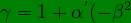+\alpha^{''}(-\beta^{2})^{2}+\alpha^{'''}(-\beta^{2})^{3} "\large \inline \dpi{120} \bg_green \bg_green \gamma=1+\alpha^{'}(-\beta^{2})+\alpha^{''}(-\beta^{2})^{2}+\alpha^{'''}(-\beta^{2})^{3}")
where
(-\frac{1}{2}-1)}{2} "\inline \dpi{120} \bg_green \alpha^{'}=-\frac{1}{2}, \alpha^{''}=\frac{(-\frac{1}{2})(-\frac{1}{2}-1)}{2}")
and
(-\frac{1}{2}-1)(-\frac{1}{2}-2)}{6} "\inline \dpi{120} \bg_green \alpha^{'''}=\frac{(-\frac{1}{2})(-\frac{1}{2}-1)(-\frac{1}{2}-2)}{6}")
therefore;

and
^{\frac{1}{2}}=1-\frac{\beta^{2}}{2}-\frac{3\beta^{4}}{8}-\frac{5\beta^{8}}{48}. "\inline \dpi{120} \bg_green \frac{1}{\gamma}=(1-\beta^{2})^{\frac{1}{2}}=1-\frac{\beta^{2}}{2}-\frac{3\beta^{4}}{8}-\frac{5\beta^{8}}{48}.")
The following are expression for
^{\pm\frac{1}{2}} "\inline \dpi{120} \bg_green \bg_green (1\pm\beta)^{\pm\frac{1}{2}}")
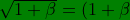^{\frac{1}{2}}=1+\frac{\beta}{2}-\frac{3\beta^{2}}{8}+\frac{5\beta^{3}}{48} \\ \frac{1}{\sqrt{1+\beta}}=(1+\beta)^{\frac{-1}{2}}=1-\frac{\beta}{2}+\frac{3\beta^{2}}{8}-\frac{5\beta^{3}}{48} \\ \sqrt{1-\beta}=(1-\beta)^{\frac{1}{2}}=1-\frac{\beta}{2}-\frac{3\beta^{2}}{8}-\frac{5\beta^{3}}{48} \\ \frac{1}{\sqrt{1-\beta}}=(1-\beta)^{\frac{-1}{2}}=1+\frac{\beta}{2}+\frac{3\beta^{2}}{8}+\frac{5\beta^{3}}{48} "\inline \dpi{120} \bg_green \bg_green \sqrt{1+\beta}=(1+\beta)^{\frac{1}{2}}=1+\frac{\beta}{2}-\frac{3\beta^{2}}{8}+\frac{5\beta^{3}}{48} \\ \frac{1}{\sqrt{1+\beta}}=(1+\beta)^{\frac{-1}{2}}=1-\frac{\beta}{2}+\frac{3\beta^{2}}{8}-\frac{5\beta^{3}}{48} \\ \sqrt{1-\beta}=(1-\beta)^{\frac{1}{2}}=1-\frac{\beta}{2}-\frac{3\beta^{2}}{8}-\frac{5\beta^{3}}{48} \\ \frac{1}{\sqrt{1-\beta}}=(1-\beta)^{\frac{-1}{2}}=1+\frac{\beta}{2}+\frac{3\beta^{2}}{8}+\frac{5\beta^{3}}{48}")
to order ;
;
 .
.
3 Doppler shift and Aberration in Special Relativity
3.1 Description of the general form of Doppler shift; recession, approach and transverse motion.
The time dilation and the Doppler shift are described here. You will notice that the usual form of time dilation given in textbooks and literature is nothing but a transverse Doppler-shift. Here we show how the Doppler transverse is always red-shifted and how the hemispheres of approach and recession are always oppositely shifted where the hemisphere of recession is entirely red-shifted. The special cases of longitudinal and transverse effects follow ipso-facto. A rigorous binomial and a basic logarithmic treatment is given.
The general form of special relativistic Lorentz transformation in terms of frequency is given in [Ref-2].
(2)}{\sqrt{1-\beta^{2}}}\quad and \quad\nu^{'}=\nu\frac{(1-\beta\cos\theta)}{\sqrt{1-\beta^{2}}} "\inline \dpi{120} \bg_green \nu=\nu^{'}\frac{(1+\beta\cos\theta)}{\sqrt{1-\beta^{2}}}\quad and \quad\nu^{'}=\nu\frac{(1-\beta\cos\theta)}{\sqrt{1-\beta^{2}}}")
the 2nd part of above equation is obtained by letting β → − β, the reciprocity of the Lorentz Transformation of inertial frames. We can see that both ν’and ν are proper frequencies and that each with respect to the other is an observed frequency. Each of the alternative cases can induce a relative change in the signs of geometric and coordinate system connections, but not the Physics. Let us rewrite the above, still in its general form;
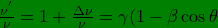=\gamma-\gamma\beta\cos\theta "\inline \dpi{120} \bg_green \frac{\nu^{'}}{\nu}=1+\frac{\Delta\nu}{\nu}=\gamma(1-\beta\cos\theta)=\gamma-\gamma\beta\cos\theta")
Now, let us apply the result of all the care we took in deriving the binomial expansion of the Lorentz factors;
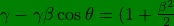-(1+\frac{\beta^{2}}{2})\beta\cos\theta "\inline \dpi{120} \bg_green \gamma-\gamma\beta\cos\theta=(1+\frac{\beta^{2}}{2})-(1+\frac{\beta^{2}}{2})\beta\cos\theta")
or
 ;
;

The above equations were obtained by using the binomial approximations to the 2nd order in β and we have now an equation to the 3rd order in β. This might change slightly if we first accommodate up-to 3rd order and then obtain our result by chopping after 3rd order. This may give rise to new terms within the 3rd order. But for most purposes β itself is very small, usually
 ,
,
e.g for satellites falling in cosmos at speeds ~ 50 times faster than jet airplanes in flight. That makes the
 .
.
We would then make an error in that order by not accommodating enough terms before the expansion.
(3)
The above equation gives the most general Doppler shift terms in the chosen order and it accommodates the transverse and longitudinal effects with angular modifications giving the general shift.

is called fractional shift in frequency. This is a very important variable and most calculations can be made very conveniently using such fractional shifts; this also relates to the fractional shifts in speed or wavelength and in time dilation/contraction. We have done another derivation, not explicitly shown in this paper, that relates the fractional shift in frequency to that in time. The result is
is equal to

in magnitude but differs by a minus sign. It is valid only when
is in itself a small fraction so binomial expansion can be used for such a fraction. In this idealized limit
 ,
,
which means a redshift is a time dilation and a blue-shift is a time contraction, speed fractions will have the same signs as time fractions:
 .
.
Thus cosθ will vary between 0 to 90 degree and we’ll accommodate the other variations of θ into sign of β. So we have 3 cases;
•(i) Doppler hemisphere of recession, θ = 0, β > 0, longitudinal Doppler effect (recession)
•(ii) Doppler hemisphere of approach, θ = 0, β < 0, longitudinal Doppler effect (approach)
•(iii) Doppler plane of intersection of hemispheres of approach and recession, θ = 90 degree, β > 0, the transverse Doppler effect.
Note that for 2nd case β < 0 is just a convention, actually 0 < β < 1, and there is a sign reversal for approach in our convention. So in all 3 cases the sign of fν and ft, the numerical sign as opposed to our algebraic sign notation, will depend on the fractions as below. We need to work out which of the two inequalities is valid, and in the following we will show that only one of them is valid in all of the cases;
(4)
Let us do some more mathematical exercise; let β be given as β = ln(α), {A short note, NOTE − 2 is to be found in section: 4 on page 1↓}. This means
+\frac{2}{ln(\alpha)}=\frac{(ln\alpha)^{2}+2}{ln(\alpha)} "\inline \dpi{120} \bg_green \beta+\frac{2}{\beta}=ln(\alpha)+\frac{2}{ln(\alpha)}=\frac{(ln\alpha)^{2}+2}{ln(\alpha)}")
under the conditions;
0 < abs(β) < 1 and ln(1) = 0
Let us now describe approach, recession and transverse motion in terms of properties of the Doppler shift in terms of β;
Approach, case (ii): ln(α) = β < 0 and Recession/Transverse, case (i), (iii): ln(α) = β > 0. So there are 2 conditions and the recognition that
^{2}>0 "\inline \dpi{120} \bg_green (ln\alpha)^{2}>0") ;
;
^{2}+2}{ln(\alpha)}\lessgtr0 "\inline \dpi{120} \bg_green \beta+\frac{2}{\beta}=\frac{2+\beta^{2}}{\beta}=\frac{(ln\alpha)^{2}+2}{ln(\alpha)}\lessgtr0")
Hence the " < " part holds for case (ii) and the " > " part holds for case (i), (iii).
For case (ii);
\Rightarrow \beta<2+\beta^{2}\Rightarrow\frac{\beta}{2}<1+\frac{\beta^{2}}{2}\Rightarrow\frac{\beta^{2}}{2}>\beta+\frac{\beta^{3}}{2} "\inline \dpi{120} \bg_green \frac{2+\beta^{2}}{\beta}<0 \hspace{2.5pt}or \hspace{2.5pt}2+\beta^{2}>\beta \hspace{2.5pt}(since \beta<0)\Rightarrow \beta<2+\beta^{2}\Rightarrow\frac{\beta}{2}<1+\frac{\beta^{2}}{2}\Rightarrow\frac{\beta^{2}}{2}>\beta+\frac{\beta^{3}}{2}")
as each time we multiply a − ve sign we must reverse the inequality.
For case (i), (iii) therefore, since in our convention,

(5)
Thus, the same inequality is valid in all cases even though the mathematical and physical conditions are different. We note here that although we derived

it is also true that

which is what we need for our purpose. We show this in our Notes.
3.2 Conclusions on nature of frequency shifts or time dilation/contraction in different regions of relative motion
Now let us return to

and
 ,
,
or equivalently,

and
 ;
;
\cos\theta\} "\inline \dpi{120} \bg_green \frac{\Delta t}{t}=f_{t}=-\{-\beta\cos\theta+\beta^{2}/2-(\beta^{3}/3)\cos\theta\}")
Case (i), (iii) can be described as:(i) → {θ = 0 degree, β > 0}, and {θ = 90 degree, β > 0} ← (iii). We deal with (i), (iii) before moving onto (ii).
• case (iii): {θ = 90 degree, β > 0}

{{We had a TYPO above/here in our earlier submitted versions to Journal acrchives, It's mentioned at the top of this page}}
This is redshift, frequency drop and time dilation. Since observed time is dilated we need to subtract
=\beta^{2}/2 "\dpi{100} \bg_green abs(f_{t})=\beta^{2}/2")
from where this time is observed and dilated, e.g. laboratory clocks, hence the − ve sign. This is also called the Transverse Doppler effect as well as time dilation. By recognizing β in terms of γ, as done in our binomial analysis, and keeping the requisite order of terms we can recognize the “footprint” of time dilation. In general, time can be either contracted or dilated. It hinges on the question “can we formalize a way of measuring time without involving processes in nature that are described by their frequencies” and the answer is NO. Hence Doppler shift is equivalent to time dilation and contraction depending on the exact situation of the motion, in other words, in reality there is no difference between time dilation/contraction and Doppler shift.
• case (i):
 ,
,
![f_{t}=-f_{\nu}=-[-\beta+\frac{\beta^{2}}{2}-\frac{\beta^{3}}{3}]](http://latex.codecogs.com/gif.latex?\inline f_{t}=-f_{\nu}=-[-\beta+\frac{\beta^{2}}{2}-\frac{\beta^{3}}{3}] "f_{t}=-f_{\nu}=-[-\beta+\frac{\beta^{2}}{2}-\frac{\beta^{3}}{3}]") ,
,  ,
,
in terms up-to 3rd order in
 ,
,
this is deliberate. We apply
Eq.(5↑): ,
,
as obtained above. Then we can see that
 .
.
The sign of ,
,  and
“primeness” of
and
“primeness” of  and
and 
are important. This will be described in a note at the end. This is redshift, frequency drop and time dilation. It is a longitudinal Doppler shift when the source and observer are receding from each other, relatively.
• case (ii):
 ,
,
 "f_{t}=-f_{\nu}=\frac{\beta^{2}}{2}-(\beta+\frac{\beta^{3}}{3})") .
.
We apply the inequality of
Eq.(5↑),
,
again. But we have to be a little careful and this applies to case (i)
above, as well. We have

which is not a Lorentz reciprocity. It represents the fact that we have chosen it to be in the lower quadrants of

whilst we require that a “line of sight” and “line of motion” extend null angle between them, see Figure 1 on page 1↓. It can be seen that the only terms that are affected are the terms that are odd in power of
as they have the cosine factors. In general
 ,
,  ,
,
but we accommodate the 3rd and 4th quadrant to

and
<1 "0<abs(\beta)<1") .
.
This leads to
 ,
,
which means a violet/blue-shift, frequency increase or time contraction. Take notice of the fact that Eq.(5↑) is still valid, as in this
quadrant with the above convention.
in this
quadrant with the above convention.
4 Notes
1. In section − III we used a convention where a primed frame is moving with respect to the unprimed at speed v = β in units of speed of light, 0 ≤ β ≤ 1. This is the convention used by [Ref-2]. In this reference ν′ is proper frequency and ν is observed frequency due to the motion/speed β. Here one has to be careful in preventing oneself from using Lorentz reciprocity inconsistently which results in accruing − ve signs. The Physics in the end has to be consistent. One rule of caution is therefore to check the signs of Δν and ν and the relative primeness of ν and ν’ which introduce additional − ve signs at unspecified points in the calculation if used incorrectly. All this could be a source of confusion under Lorentz reciprocation.
2. One can prove the above results without using ln() by just employing the properties of numbers, viz the square of any real number is always positive. But having ln() may be useful if one intends to study a functional form of β. It is widely customary in Relativity to have logarithmic functions and we think it is very useful for generalization purposes.
3. We use in our analysis the fact that
in the limit of
 .
.
This is a known fact. We show here how we arrive at this conclusion ourselves, independent of any assumptions other than elementary. By elementary definition

and

we deduce:
/\frac{1}{t}=\frac{t-t'}{t'}=-\frac{\triangle t}{t'} "\inline \dpi{120} \bg_green \frac{\triangle\nu}{\nu}=\frac{\nu'-\nu}{\nu}=\left(\frac{1}{t'}-\frac{1}{t}\right)/\frac{1}{t}=\frac{t-t'}{t'}=-\frac{\triangle t}{t'}") .
.
Then,
 .
.
Because

we have
 ,
,
it follows then from

that
 ,
,
so

\frac{t}{\nu}=-\frac{\triangle t}{\triangle\nu}. "\inline \dpi{120} \bg_green \left(1+\frac{\triangle t}{t}\right)\frac{t}{\nu}=-\frac{\triangle t}{\triangle\nu}.")

=-\frac{\triangle t}{\triangle\nu}. "\inline \dpi{120} \bg_green \frac{1}{\nu}\left(t+\triangle t\right)=-\frac{\triangle t}{\triangle\nu}.")


So,
(6)
This leads to
}{\triangle\nu/\nu}\right] "\inline \dpi{120} \bg_green \frac{t}{\triangle t}=-\left[\frac{1+\left(\triangle\nu/\nu\right)}{\triangle\nu/\nu}\right]")
So we have;
}\right]. "\inline \dpi{120} \bg_green \frac{\triangle t}{t}=-\left[\frac{\triangle\nu/\nu}{1+\left(\triangle\nu/\nu\right)}\right].") (7)
(7)
4. Here we show how

follows from

We write
=\beta(1+\frac{\beta^{2}}{3}+\frac{\beta^{2}}{2}-\frac{\beta^{2}}{3})=\beta(1+\frac{\beta^{2}}{3}+\frac{\beta^{2}}{6})=\beta(1+\frac{\beta^{2}}{3})+\frac{\beta^{3}}{6} "\inline \dpi{120} \bg_green \hspace{2.5pt}\beta+\frac{\beta^{3}}{2}=\beta(1+\frac{\beta^{2}}{2})=\beta(1+\frac{\beta^{2}}{3}+\frac{\beta^{2}}{2}-\frac{\beta^{2}}{3})=\beta(1+\frac{\beta^{2}}{3}+\frac{\beta^{2}}{6})=\beta(1+\frac{\beta^{2}}{3})+\frac{\beta^{3}}{6}")
as

this implies
+\frac{\beta^{3}}{6} "\inline \dpi{120} \bg_green \frac{\beta^{2}}{2}>\beta(1+\frac{\beta^{2}}{3})+\frac{\beta^{3}}{6}") ,
,
if

which implies
 "\inline \dpi{120} \bg_green \frac{\beta^{2}}{2}>\beta(1+\frac{\beta^{2}}{3})")
if

L.H.S. is +ve and R.H.S. is -ve which again implies
since both terms of R.H.S. are -ve.
5. We already mentioned this but summarize again: There is a cosθ multiplied to odd powers of β which comes in − ve sign relative to the even powers in the general frequency shift. For our considerations 0 < θ < 900, 0 < cosθ < 1,
\Rightarrow\frac{\beta^{2}}{2}>\beta\cos\theta+(\frac{\beta^{3}}{3})\cos\theta "\inline \dpi{120} \bg_green \frac{\beta^{2}}{2}>\beta+(\frac{\beta^{3}}{3})\Rightarrow\frac{\beta^{2}}{2}>\beta\cos\theta+(\frac{\beta^{3}}{3})\cos\theta")
always. Hence the hemisphere of approach is always oppositely shifted with respect to the hemisphere of recession; recession being red-shifted, approach must be blue in the entire hemisphere. At the intersection the

and odd terms vanishes to order of
 .
.
We intuit that this is valid to all higher powers as well. Therefore a transverse shift is always + ve or red-shifted by an amount,

and with the correct binomial-fractions it applies to all higher even powers of β.
6. The aberration such as that of star-light is the angular deflection caused by the relative motion of the source and observer. If our detectors are mounted on moving frames {e.g. earth itself} even very small speed differences cause the frequency to differ due to the angle extended by such relative velocity. The aberration of an order β is given by β = tanθ. For small values of β therefore, the fractional speed increment can be measured by the fractional angular deflection, and these are equal. We have not studied this in detail hence we are not giving any results here. But one can see that when there is a β the Lorentz transformations of the θ or tanθ can be treated as it has been in this paper.
7. The fractional shifts fν can themselves be binomially expanded when they are small, which is so for small values of β. It is then equal to the fractional shifts in time ft and fλ etc, except for a relative − ve sign in case of ft. So there are two scenarios. In the first fν has to be expanded to higher orders binomially, in-case of small β-values. This will perhaps be rigorous, but unnecessary, since we will otherwise incur errors of only inconsequential proportion. In the 2nd scenario, in-case β↠1, we have to review by some other method to find what the consequences are. In this latter case the binomial expansion is still valid, since β ≤ 1, always. But, the relation between fractional shifts in the variables may need to be reviewed.
8. The fractional increments or reduction in speed,

is related, in the case of small values of
,
by a factor of 2 to the same. In other words,
 .
.
That is so, assuming that the final absolute shifts in frequency are shifts by the square of the speed. e.g. in telemetry of celestial objects the frequency used will give different results by this factor for the same frequency, if this relation between fν and fv is not readily recognized.
9. A note on terminology and nature of the factors β and γ. We ask ourselves a fundamental notional question, which is more fundamental β or γ? One defines β from the basic speed-of-light perspective and then defines γ based on this definition because the latter makes calculations easier as the β’s appear in denominator, in numerator, inside square-roots and inside particle detectors and where-not. It is a serious factual observation that inside a particle detector, like in the case of the recent OPERA [Ref-3] experiment, one must proceed from basic relativistic equations and gradually factor in the contributions from various sources if one wants to see the total effect in a consistent way, Quantum Mechanics included. So defining these two parameters instead of just one would make life easier for concise studies. If β > 1 it poses problems to the mathematical nature of Relativity because what comes out is a complex number γ, and only Quantum Mechanics can deal with such a problem, which is why it is interesting to note that the answer to the OPERA anomaly is likely inherent here; because Δβ = 7.5 km ⁄ s = 25 ppm in terms of speed-of-light, and without the application of Quantum Mechanics, this is a pointer to a “non-physical” character of Relativity as stated above.
On terminology we would like to further note that the “Lorentz factor” is the most general terminology as it defines both β and γ, when we say β: speed factor is enough, although it is somewhat casual. When we say γ: Lorentz factor, Lorentz boost, speed factor, boost factor, or simply boost, all work to define suitably. Actually β and γ are equivalents as implicitly pointed out above in their definitions, hence all of the terminology is correct in any of the cases. So a β can be said to be a boost-factor as well; once one is defined or measured, the other is immediately known in practice. In theory it is β that is more fundamental, −we can see this just from intuitive understanding and the correspondence principle, as there never was a γ explicitly prior to relativistic formulations, but there was a β, just by the fact that people compared ratios of various velocities: “How fast is object A compared to object B”, a ratio of their speeds deals with this; “how fast is object A or B compared to light”; that ratio is known as β and the relativistic formulation 0 ≤ β ≤ 1 reminds us that nothing travels faster than light, hence this ratio is always slated to be a fraction where as γ is not.
10. In Figure2 on page 1↓ we have defined a sphere of relative motion, (- drawn in a blue-dotted pattern -), whose center is the position where an observer or detector is located. The L.O.S. or line of sight extends from the detector by a blue line. We show 3 trajectories of actual importance.
•The 1st one is a meteor or crashing satellite falling e.g. towards Earth’s surface, lies in the region of approach as gradually its distance is reduced from the earth-centered reference.
•The 2nd one is a circle or sphere which serves as a “sphere of reference” concentric with many such spheres of reference. But, we can also chose one of these circle/sphere as one which defines the circular orbits of some satellites, such as the orbit of most GPS satellites. The speed vector will then be transverse/tangential to the circle or sphere of reference. Hence this defines the intersection of two hemispheres, which add to give us the sphere of relative motion. We may call it the “sphere of relative motion” as it is this sphere that contains a speed-vector or trajectory segment of the actual motion.
•In the 3rd scenario the speed vector or radial velocity vector of a hyperbolic motion is also shown; this one belongs to the hemisphere of recession, as the trajectory implies a configuration of gradually larger radial separation. Note that this only describes an instantaneous situation as depicted in this diagram. Also for a hyperbolic trajectory where an object is approaching us from below or above, the region represented by a segment of the hyperbola will lie in the hemisphere of approach instead of recession.
By the same reasoning, when we have accumulated enough change from the instantaneous situation, we need to define larger or smaller circles/spheres of reference and spheres of relative motion. We call it the sphere of relative motion as the L.O.S. defines the “relativeness” of the speed-vectors which then define which region is a region of approach and which is a region of recession relative to the references.

Figure 1 The time dilation/contraction effects as frequency red-shift/blue-shift, shown for above configuration.

Figure 2 This diagram explains our terminology, sphere of reference and sphere of relative motion. L.O.S. = Line Of Sight. See NOTE − 9 in section 4↑.
5 Summary/Conclusion
Our definition of special notions of reference of observation and reference of actual motion path enables an investigation of important relativistic effects. We have deduced from an application of the binomial theorem and properties of either logarithmic or real numbers that Doppler shift and time dilation of Special Relativity are oppositely signed in two hemispheres, which naturally define where the motion trajectory lies with respect to the observer and the line of sight. An application on aberration of special relativistic recession and approach is also inherent here. The analysis draws on very basic, yet non-trivial, and not-so-often cited facts of Relativity. This paper serves as an explicit reminder of the mathematical apparatus of Relativity. Thus, the concept and methodology presented in this paper should be applicable to a wide variety of investigations, especially where one seeks accuracy to very high powers of β, through binomial expansion. We have developed this paper in a generalized treatment suitable for future reference.
We are thankful to the free world for the resources which enabled us to discuss our ideas and communicate the research. In special we would like to mention free software from various sources such as source-forge and Lyx, X-fig, Google-docs repository and share, and a social site where we frequently find it very easy to make our communication: Face Book and Word-press blog-site. These sites have been a constant and supportive source for our communication without which the communication and brainstorming prior to professional sharing was not possible for us. This research was in part supported by i3tex and the Willgood institute. Both authors also thank their families for a remarkable support they have enjoyed from their families. Furthermore, we are grateful for the valuable feedback provided by Professor Giovanni Modanese.
References
[1] G.Arfken, H.Weber, "Binomial Theorem", 6th Indian edition, chapter 5.6, (2009).
[2] R.Resnick, "Introduction to Special Relativity", (1968).
[3] The OPERA Collaboration, “Measurement of the neutrino velocity with the OPERA detector in the CNGS beam”, arXiv:1109.4897v1 [hep-ex], (2011).
--------------------------------------------------------------------------------
Document generated by eLyXer 1.2.3 (2011-08-31) on 2012-01-17T23:05:24.184000
FYI-2: our paper version on Philica.com, cited below, has some errors in Note-3. The Note-3 in this html version, the UTexas Math-Phys Archive version and the HAL INRIA version are correct. We have communicated with Philica to have Note-3 replaced with the correct version.
FYI-3: One obvious typographical error in earlier versions has been fixed.
((should actually be))
The above typo is not corrected in any archive copies.
If you want to cite our version
Citation: "Time dilation have opposite signs in hemispheres of recession and approach.", Manmohan Dash and Mikael Franzen, Communicating Science, January 17, 2011, publisher: Invariance Publishing House, MDash Foundation
Our citations might slightly change depending on exact source where we placed our ideas first. eg we may want to cite our online journals "Various Musings" if we formalize it and make it permanent.
Link to permaweblink in citation or copy/archive material as it is with Creative Commons and other copyrights in this web-site in mind: permaweblink
Time dilation have opposite signs in hemispheres of recession and approach.
Manmohan Dash and Mikael Franzen
First publicized/Available Online (Link to other articles; Article-1, Article-2): January 17, 2011 or earlier
Alternative versions
i. Dash, M. & Franzén, M. (2012). Time dilation have opposite signs in hemispheres of recession and approach. PHILICA.COM Article number 312.
ii. University of Texas, Mathematical Physics, Mathematical Physics Preprint Archive mp_arc
iii. Open Access on HAL INRIA (ps, pdf) HAL-Inria; Link to the pdf PDF version of the paper
Time dilation have opposite signs in hemispheres of recession and approach.
Manmohan Dash
mdash@vt.edu
manmohan.dash@willgood.org
i. Informal association with Willgood institute, registered in Sweden, author’s mail: Mahisapat, Dhenkanal, Odisha, India, 759001
ii. previously affiliated with VT, USA and KEK, Japan.
Mikael Franzén
mikael.franzen@willgood.org
mikael.franzen@i3tex.com
i. Willgood Institute, Luckvägen 5, 517 37 Bollebygd, Sweden
ii. i3tex AB, Klippan 1A , 414 51 Gothenburg, Sweden
Abstract
In this paper we give a detailed analysis of the factual observation that time dilation or Doppler shift of frequency are oppositely signed relative to our line of sight in different regions of motion. We show that this depends on how these regions are connected to the actual path of motion and to the location of the observer/detector. For a static globe or circle/sphere of reference, we define two hemispheres; shifts will be red-shifted in the hemisphere of recession and blue-shifted, or violet shifted, in the hemisphere of approach, a fact which is not often mentioned. Indeed, it is a complete sphere where the motion can take place with respect to the line-of-sight, which we have studied in this paper, not just the direction of motion along a certain specific path. The transverse and longitudinal effects are special cases of this general effect. The transverse effect is always red-shifted consistent with the known effect of Relativity and it lies at the intersection of the hemispheres of approach and recession. By saying moving clocks run slower we conveniently forget this important effect. They also run faster, in the hemisphere of approach. We demonstrate this important result from the basic principles of the Special Theory of Relativity.
Keywords: Time Dilation, Special Relativity, Doppler Shift, Binomial Expansion, Celestial trajectories and Time dilation
1 Introduction
We perform a detailed analysis of how relative to the line-of-sight a general motion of a source and equivalently an observer will affect observation of time dilation and Doppler shift. We use only two main references, so we mention this fact here; [Ref-1] and [Ref-2]. It is a straightforward but non-trivial analysis. It applies to any situation where one would like to have a binomial expansion of the Lorentz factors γ and β to any desired degree of accuracy by retaining terms up-to one’s requirements. This will be useful in many studies.
Let us now define the context in which we have used terminology like “sphere of relative motion”, “hemispheres of recession” and “spheres of reference”; see Figure 1↓ and Figure 2↓. Our definition is a natural extension of the concept of reference frames. This is helpful towards identification of the relations of different parts to each other in the problem. Simply put, one defines two spheres/circles, the first one is a sphere of reference whose center is where a detector or origin of reference is located. The detector can also be placed e.g. at the surface of another object whose center is at the center of this reference. Any concentric sphere that encloses or excludes a segment of the trajectory of another object is also a sphere of reference. Now a second sphere of reference can be defined. This second sphere will encompass a segment of the trajectory path so the path lies in either the lower or upper hemisphere with respect to the line of sight. Let us call it a sphere of relative motion as it defines whether an object is receding away from, or approaching the center of reference. The upper hemisphere of this second sphere, where an object is gradually moving away from the reference point, defined at the center of the first sphere, can be called a hemisphere of recession. On the other hand, if the object is in the lower hemisphere of the second sphere, we can call it a hemisphere of approach, as the object will gradually approach the center of reference. One must note that these spheres are not very arbitrary in nature, but rather, dependent on the specific nature of the trajectories, e.g. a satellite orbiting a planet in a circle will naturally always traverse the intersection of the two hemispheres, so it is a transverse motion to the line of sight. In hyperbolic motion, such as that of a flyby satellite moving away from a planet towards some other destination, part of the motion lies in the upper hemisphere or the hemisphere of recession. When dealing with earthbound motion, such as before perigee, the point of closest approach to earth, the opposite is true. The segment of the trajectory is naturally proportional to the radial speed vector. The radial − speed − vecor is very important for any study of celestial applications. Similarly a meteor falling towards Earth always lies in the hemisphere of approach. One sees that one can cautiously adjust the sphere of reference and the sphere of relative motion so that there is no ambiguity in the situation. Only then can one consistently apply the laws of Relativity, such as those that govern time dilation and Doppler shift of frequencies.
We also note as a reminder of convenience that the transverse effects are always 2nd order in speed of recession and the longitudinal effects are 1st and 3rd order in terms of the Lorentz factor, β. Higher order terms appear in the same pattern. Transverse effects contain β2 and β4 and longitudinal effects contain alternative odd terms given by factors from binomial expansion as presented in our analysis.
The general case is accommodated by cosines of a suitable angle, which appear only in the orders of odd power terms. The analysis is valid for 0 ≤ abs(β) ≤ 1, where abs stands for the modulus of a number or the regular absolute value function. The relation between fractional frequency shift fν and fractional time dilation or contraction ft related to fν are computed here and these are equal in their modulus. This is the case when the fν’s are small. When they are not small, additional review is necessary for the relation between the f’s in ν, t, λ and v. We note that this also follows a binomial analysis like the one presented in this paper, because the fν’s are fractions.
2 Binomial Theorem
The form and properties of binomial expansion is given in [Ref-1] for: − 1 < x < 1
(1)
By using the above, we derive the Lorentz factors γ and its products with β or its functions, and any powers in the following steps,
expanding in the power of
where
and
therefore;
and
The following are expression for
to order
3 Doppler shift and Aberration in Special Relativity
3.1 Description of the general form of Doppler shift; recession, approach and transverse motion.
The time dilation and the Doppler shift are described here. You will notice that the usual form of time dilation given in textbooks and literature is nothing but a transverse Doppler-shift. Here we show how the Doppler transverse is always red-shifted and how the hemispheres of approach and recession are always oppositely shifted where the hemisphere of recession is entirely red-shifted. The special cases of longitudinal and transverse effects follow ipso-facto. A rigorous binomial and a basic logarithmic treatment is given.
The general form of special relativistic Lorentz transformation in terms of frequency is given in [Ref-2].
(2)
the 2nd part of above equation is obtained by letting β → − β, the reciprocity of the Lorentz Transformation of inertial frames. We can see that both ν’and ν are proper frequencies and that each with respect to the other is an observed frequency. Each of the alternative cases can induce a relative change in the signs of geometric and coordinate system connections, but not the Physics. Let us rewrite the above, still in its general form;
Now, let us apply the result of all the care we took in deriving the binomial expansion of the Lorentz factors;
or
e.g for satellites falling in cosmos at speeds ~ 50 times faster than jet airplanes in flight. That makes the
We would then make an error in that order by not accommodating enough terms before the expansion.
(3)
The above equation gives the most general Doppler shift terms in the chosen order and it accommodates the transverse and longitudinal effects with angular modifications giving the general shift.
is called fractional shift in frequency. This is a very important variable and most calculations can be made very conveniently using such fractional shifts; this also relates to the fractional shifts in speed or wavelength and in time dilation/contraction. We have done another derivation, not explicitly shown in this paper, that relates the fractional shift in frequency to that in time. The result is
is equal to
in magnitude but differs by a minus sign. It is valid only when
is in itself a small fraction so binomial expansion can be used for such a fraction. In this idealized limit
which means a redshift is a time dilation and a blue-shift is a time contraction, speed fractions will have the same signs as time fractions:
Thus cosθ will vary between 0 to 90 degree and we’ll accommodate the other variations of θ into sign of β. So we have 3 cases;
•(i) Doppler hemisphere of recession, θ = 0, β > 0, longitudinal Doppler effect (recession)
•(ii) Doppler hemisphere of approach, θ = 0, β < 0, longitudinal Doppler effect (approach)
•(iii) Doppler plane of intersection of hemispheres of approach and recession, θ = 90 degree, β > 0, the transverse Doppler effect.
Note that for 2nd case β < 0 is just a convention, actually 0 < β < 1, and there is a sign reversal for approach in our convention. So in all 3 cases the sign of fν and ft, the numerical sign as opposed to our algebraic sign notation, will depend on the fractions as below. We need to work out which of the two inequalities is valid, and in the following we will show that only one of them is valid in all of the cases;
(4)
Let us do some more mathematical exercise; let β be given as β = ln(α), {A short note, NOTE − 2 is to be found in section: 4 on page 1↓}. This means
under the conditions;
0 < abs(β) < 1 and ln(1) = 0
Let us now describe approach, recession and transverse motion in terms of properties of the Doppler shift in terms of β;
Approach, case (ii): ln(α) = β < 0 and Recession/Transverse, case (i), (iii): ln(α) = β > 0. So there are 2 conditions and the recognition that
Hence the " < " part holds for case (ii) and the " > " part holds for case (i), (iii).
For case (ii);
as each time we multiply a − ve sign we must reverse the inequality.
For case (i), (iii) therefore, since in our convention,
(5)
Thus, the same inequality is valid in all cases even though the mathematical and physical conditions are different. We note here that although we derived
it is also true that
which is what we need for our purpose. We show this in our Notes.
3.2 Conclusions on nature of frequency shifts or time dilation/contraction in different regions of relative motion
Now let us return to
and
or equivalently,
and
Case (i), (iii) can be described as:(i) → {θ = 0 degree, β > 0}, and {θ = 90 degree, β > 0} ← (iii). We deal with (i), (iii) before moving onto (ii).
• case (iii): {θ = 90 degree, β > 0}
{{We had a TYPO above/here in our earlier submitted versions to Journal acrchives, It's mentioned at the top of this page}}
This is redshift, frequency drop and time dilation. Since observed time is dilated we need to subtract
from where this time is observed and dilated, e.g. laboratory clocks, hence the − ve sign. This is also called the Transverse Doppler effect as well as time dilation. By recognizing β in terms of γ, as done in our binomial analysis, and keeping the requisite order of terms we can recognize the “footprint” of time dilation. In general, time can be either contracted or dilated. It hinges on the question “can we formalize a way of measuring time without involving processes in nature that are described by their frequencies” and the answer is NO. Hence Doppler shift is equivalent to time dilation and contraction depending on the exact situation of the motion, in other words, in reality there is no difference between time dilation/contraction and Doppler shift.
• case (i):
in terms up-to 3rd order in
this is deliberate. We apply
Eq.(5↑):
as obtained above. Then we can see that
The sign of
are important. This will be described in a note at the end. This is redshift, frequency drop and time dilation. It is a longitudinal Doppler shift when the source and observer are receding from each other, relatively.
• case (ii):
We apply the inequality of
Eq.(5↑),
again. But we have to be a little careful and this applies to case (i)
above, as well. We have
which is not a Lorentz reciprocity. It represents the fact that we have chosen it to be in the lower quadrants of
whilst we require that a “line of sight” and “line of motion” extend null angle between them, see Figure 1 on page 1↓. It can be seen that the only terms that are affected are the terms that are odd in power of
as they have the cosine factors. In general
but we accommodate the 3rd and 4th quadrant to
and
This leads to
which means a violet/blue-shift, frequency increase or time contraction. Take notice of the fact that Eq.(5↑) is still valid, as
4 Notes
1. In section − III we used a convention where a primed frame is moving with respect to the unprimed at speed v = β in units of speed of light, 0 ≤ β ≤ 1. This is the convention used by [Ref-2]. In this reference ν′ is proper frequency and ν is observed frequency due to the motion/speed β. Here one has to be careful in preventing oneself from using Lorentz reciprocity inconsistently which results in accruing − ve signs. The Physics in the end has to be consistent. One rule of caution is therefore to check the signs of Δν and ν and the relative primeness of ν and ν’ which introduce additional − ve signs at unspecified points in the calculation if used incorrectly. All this could be a source of confusion under Lorentz reciprocation.
2. One can prove the above results without using ln() by just employing the properties of numbers, viz the square of any real number is always positive. But having ln() may be useful if one intends to study a functional form of β. It is widely customary in Relativity to have logarithmic functions and we think it is very useful for generalization purposes.
3. We use in our analysis the fact that
in the limit of
This is a known fact. We show here how we arrive at this conclusion ourselves, independent of any assumptions other than elementary. By elementary definition
and
we deduce:
Then,
Because
we have
it follows then from
that
so
So,
This leads to
So we have;
4. Here we show how
follows from
We write
as
this implies
if
which implies
if
L.H.S. is +ve and R.H.S. is -ve which again implies
since both terms of R.H.S. are -ve.
5. We already mentioned this but summarize again: There is a cosθ multiplied to odd powers of β which comes in − ve sign relative to the even powers in the general frequency shift. For our considerations 0 < θ < 900, 0 < cosθ < 1,
always. Hence the hemisphere of approach is always oppositely shifted with respect to the hemisphere of recession; recession being red-shifted, approach must be blue in the entire hemisphere. At the intersection the
and odd terms vanishes to order of
We intuit that this is valid to all higher powers as well. Therefore a transverse shift is always + ve or red-shifted by an amount,
and with the correct binomial-fractions it applies to all higher even powers of β.
6. The aberration such as that of star-light is the angular deflection caused by the relative motion of the source and observer. If our detectors are mounted on moving frames {e.g. earth itself} even very small speed differences cause the frequency to differ due to the angle extended by such relative velocity. The aberration of an order β is given by β = tanθ. For small values of β therefore, the fractional speed increment can be measured by the fractional angular deflection, and these are equal. We have not studied this in detail hence we are not giving any results here. But one can see that when there is a β the Lorentz transformations of the θ or tanθ can be treated as it has been in this paper.
7. The fractional shifts fν can themselves be binomially expanded when they are small, which is so for small values of β. It is then equal to the fractional shifts in time ft and fλ etc, except for a relative − ve sign in case of ft. So there are two scenarios. In the first fν has to be expanded to higher orders binomially, in-case of small β-values. This will perhaps be rigorous, but unnecessary, since we will otherwise incur errors of only inconsequential proportion. In the 2nd scenario, in-case β↠1, we have to review by some other method to find what the consequences are. In this latter case the binomial expansion is still valid, since β ≤ 1, always. But, the relation between fractional shifts in the variables may need to be reviewed.
8. The fractional increments or reduction in speed,
is related, in the case of small values of
by a factor of 2 to the same. In other words,
That is so, assuming that the final absolute shifts in frequency are shifts by the square of the speed. e.g. in telemetry of celestial objects the frequency used will give different results by this factor for the same frequency, if this relation between fν and fv is not readily recognized.
9. A note on terminology and nature of the factors β and γ. We ask ourselves a fundamental notional question, which is more fundamental β or γ? One defines β from the basic speed-of-light perspective and then defines γ based on this definition because the latter makes calculations easier as the β’s appear in denominator, in numerator, inside square-roots and inside particle detectors and where-not. It is a serious factual observation that inside a particle detector, like in the case of the recent OPERA [Ref-3] experiment, one must proceed from basic relativistic equations and gradually factor in the contributions from various sources if one wants to see the total effect in a consistent way, Quantum Mechanics included. So defining these two parameters instead of just one would make life easier for concise studies. If β > 1 it poses problems to the mathematical nature of Relativity because what comes out is a complex number γ, and only Quantum Mechanics can deal with such a problem, which is why it is interesting to note that the answer to the OPERA anomaly is likely inherent here; because Δβ = 7.5 km ⁄ s = 25 ppm in terms of speed-of-light, and without the application of Quantum Mechanics, this is a pointer to a “non-physical” character of Relativity as stated above.
On terminology we would like to further note that the “Lorentz factor” is the most general terminology as it defines both β and γ, when we say β: speed factor is enough, although it is somewhat casual. When we say γ: Lorentz factor, Lorentz boost, speed factor, boost factor, or simply boost, all work to define suitably. Actually β and γ are equivalents as implicitly pointed out above in their definitions, hence all of the terminology is correct in any of the cases. So a β can be said to be a boost-factor as well; once one is defined or measured, the other is immediately known in practice. In theory it is β that is more fundamental, −we can see this just from intuitive understanding and the correspondence principle, as there never was a γ explicitly prior to relativistic formulations, but there was a β, just by the fact that people compared ratios of various velocities: “How fast is object A compared to object B”, a ratio of their speeds deals with this; “how fast is object A or B compared to light”; that ratio is known as β and the relativistic formulation 0 ≤ β ≤ 1 reminds us that nothing travels faster than light, hence this ratio is always slated to be a fraction where as γ is not.
10. In Figure2 on page 1↓ we have defined a sphere of relative motion, (- drawn in a blue-dotted pattern -), whose center is the position where an observer or detector is located. The L.O.S. or line of sight extends from the detector by a blue line. We show 3 trajectories of actual importance.
•The 1st one is a meteor or crashing satellite falling e.g. towards Earth’s surface, lies in the region of approach as gradually its distance is reduced from the earth-centered reference.
•The 2nd one is a circle or sphere which serves as a “sphere of reference” concentric with many such spheres of reference. But, we can also chose one of these circle/sphere as one which defines the circular orbits of some satellites, such as the orbit of most GPS satellites. The speed vector will then be transverse/tangential to the circle or sphere of reference. Hence this defines the intersection of two hemispheres, which add to give us the sphere of relative motion. We may call it the “sphere of relative motion” as it is this sphere that contains a speed-vector or trajectory segment of the actual motion.
•In the 3rd scenario the speed vector or radial velocity vector of a hyperbolic motion is also shown; this one belongs to the hemisphere of recession, as the trajectory implies a configuration of gradually larger radial separation. Note that this only describes an instantaneous situation as depicted in this diagram. Also for a hyperbolic trajectory where an object is approaching us from below or above, the region represented by a segment of the hyperbola will lie in the hemisphere of approach instead of recession.
By the same reasoning, when we have accumulated enough change from the instantaneous situation, we need to define larger or smaller circles/spheres of reference and spheres of relative motion. We call it the sphere of relative motion as the L.O.S. defines the “relativeness” of the speed-vectors which then define which region is a region of approach and which is a region of recession relative to the references.

Figure 1 The time dilation/contraction effects as frequency red-shift/blue-shift, shown for above configuration.

Figure 2 This diagram explains our terminology, sphere of reference and sphere of relative motion. L.O.S. = Line Of Sight. See NOTE − 9 in section 4↑.
5 Summary/Conclusion
Our definition of special notions of reference of observation and reference of actual motion path enables an investigation of important relativistic effects. We have deduced from an application of the binomial theorem and properties of either logarithmic or real numbers that Doppler shift and time dilation of Special Relativity are oppositely signed in two hemispheres, which naturally define where the motion trajectory lies with respect to the observer and the line of sight. An application on aberration of special relativistic recession and approach is also inherent here. The analysis draws on very basic, yet non-trivial, and not-so-often cited facts of Relativity. This paper serves as an explicit reminder of the mathematical apparatus of Relativity. Thus, the concept and methodology presented in this paper should be applicable to a wide variety of investigations, especially where one seeks accuracy to very high powers of β, through binomial expansion. We have developed this paper in a generalized treatment suitable for future reference.
We are thankful to the free world for the resources which enabled us to discuss our ideas and communicate the research. In special we would like to mention free software from various sources such as source-forge and Lyx, X-fig, Google-docs repository and share, and a social site where we frequently find it very easy to make our communication: Face Book and Word-press blog-site. These sites have been a constant and supportive source for our communication without which the communication and brainstorming prior to professional sharing was not possible for us. This research was in part supported by i3tex and the Willgood institute. Both authors also thank their families for a remarkable support they have enjoyed from their families. Furthermore, we are grateful for the valuable feedback provided by Professor Giovanni Modanese.
References
[1] G.Arfken, H.Weber, "Binomial Theorem", 6th Indian edition, chapter 5.6, (2009).
[2] R.Resnick, "Introduction to Special Relativity", (1968).
[3] The OPERA Collaboration, “Measurement of the neutrino velocity with the OPERA detector in the CNGS beam”, arXiv:1109.4897v1 [hep-ex], (2011).
--------------------------------------------------------------------------------
Document generated by eLyXer 1.2.3 (2011-08-31) on 2012-01-17T23:05:24.184000
Subscribe to:
Posts (Atom)